Blogs | Page 313 | Paleontology World

Blogs

Ceratosaurus

Saturday, November 19, 2016

Artist's impression of C. nasicornis

Ceratosaurus was a large predatory theropod dinosaur from the Late Jurassic Period (Kimmeridgian to Tithonian), found in the Morrison Formation of North America, and the Lourinhã Formation of Portugal (and possibly the Tendaguru Formation in Tanzania). It was characterized by large jaws with blade-like teeth, a large, blade-like horn on the snout and a pair of hornlets over the eyes. The forelimbs were powerfully built but very short. The bones of the sacrum were fused (synsacrum) and the pelvic bones were fused together and to this structure (i.e. similar to modern birds). A row of small osteoderms was present down the middle of the back.

Ceratosaurus, at first glance, looked like a fairly typical theropod, however its skull was quite large in proportion to the rest of its body, and large nasal and brow horns and possessed a prominent nose horn formed from protuberances of the nasal bones. In addition to the large nasal horn, Ceratosaurus possessed smaller hornlike ridges in front of each eye, similar to those of Allosaurus, these ridges were formed by enlargement of the lacrimal bones. Uniquely among theropods, Ceratosaurus possessed dermal armor, in the form of small osteoderms running down the middle of its back. Its tail comprised about half of the body’s total length and was thin and flexible with high vertebral spines.

The type specimen was an individual about 18 feet (5.5 m) long; it is not clear whether this animal was fully grown. David B. Norman (1985) estimated that the maximum length of Ceratosaurus was 20 ft (6.1 m), an assessment supported by a particularly large Ceratosaurus specimen from the Cleveland-Lloyd Dinosaur Quarry (UMNH 5728), discovered in the mid-1960s, which may have been 22 ft (6.7 m) long assuming similar proportions to the holotype.

Ceratosaurus is known from the Cleveland-Lloyd Dinosaur Quarry in central Utah and the Dry Mesa Quarry in Colorado. The type species, described by O. C. Marsh in 1884 and redescribed by Gilmore in 1920, is Ceratosaurus nasicornis. The first skeleton was excavated by rancher Marshall Parker Felch in 1883.

Size of two specimens compared to a human, with the holotype of Ceratosaurus nasicornis (USNM 4735) in orange and a larger specimen (UMNH VP 5278) in blue

Ceratosaurus gives its name to the Ceratosauria, a clade of theropod dinosaurs that diverged early from the evolutionary lineage leading to modern birds. Within the Ceratosauria, some paleontologists proposed it to be most closely related to Genyodectes from Argentina, which shares the strongly elongated teeth. The geologically older genus Proceratosaurus from England, although originally described as a presumed antecedent of Ceratosaurus, was later found to be unrelated. Ceratosaurus shared its habitat with other large theropod genera including Torvosaurus and Allosaurus, and it has been suggested that these theropods occupied different ecological niches to reduce competition. Ceratosaurus may have preyed upon plant-eating dinosaurs, although some paleontologists suggested that it hunted aquatic prey such as fish. The nasal horn was probably not used as a weapon as was originally suggested by Marsh, but more likely was used solely for display.

Ceratosaurus followed the body plan typical for large theropod dinosaurs. A biped, it moved on powerful hind legs, while its arms were reduced in size. Specimen USNM 4735, the first discovered skeleton and holotype of Ceratosaurus nasicornis, was an individual 5.3 m (17 ft) or 5.69 m (18.7 ft) in length according to separate sources. Whether this animal was fully grown is not clear. Othniel Charles Marsh, in 1884, suggested that this specimen weighed about half as much as the contemporary Allosaurus. In more recent accounts, this was revised to 418 kilograms (922 lb), 524 kg (1,155 lb), or 670 kg (1,480 lb). Three additional skeletons discovered in the latter half of the 20th century were substantially larger. The first of these, UMNH VP 5278, was informally estimated by James Madsen to have been around 8.8 m (29 ft) long, but was later estimated at 7 m (23 ft) in length. Its weight was calculated at 980 kg (2,160 lb), 452 kg (996 lb), and 700 kg (1,540 lb) in separate works. The second skeleton, MWC 1, was somewhat smaller than UMNH VP 5278 and might have been 275 kg (606 lb) in weight. The third, yet undescribed, specimen BYUVP 12893 was claimed to be the largest yet discovered, although estimates have not been published. Another specimen (ML 352), discovered in Portugal in 2000, was estimated at 6 m (20 ft) in length and 600 kg (1,320 lb) in weight.

Ceratosaurus

Classification

In his original description of the Ceratosaurus nasicornis holotype and subsequent publications, Marsh noted a number of characteristics that were unknown in all other theropods known at the time. Two of these features, the fused pelvis and fused metatarsus, were known from modern-day birds, and according to Marsh, clearly demonstrate the close relationship between the latter and dinosaurs. To set the genus apart from Allosaurus, Megalosaurus, and coelurosaurs, Marsh made Ceratosaurus the only member of both a new family, the Ceratosauridae, and a new infraorder, the Ceratosauria. This was questioned in 1892 by Edward Drinker Cope, Marsh's rival in the Bone Wars, who argued that distinctive features such as the nasal horn merely showed that C. nasicornis was a distinct species, but were insufficient to justify a distinct genus. Consequently, he assigned C. nasicornis to the genus Megalosaurus, creating the new combination Megalosaurus nasicornis.

Although Ceratosaurus was retained as a distinct genus in all subsequent analyses, its relationships remained controversial during the following century. Both the Ceratosauridae and Ceratosauria were not widely accepted, with only few and poorly known additional members identified. Over the years, separate authors classified Ceratosaurus within the Deinodontidae, the Megalosauridae, the Coelurosauria, the Carnosauria, and the Deinodontoidea. In his 1920 revision, Gilmore argued that the genus was the most basal theropod known from after the Triassic, so not closely related to any other contemporary theropod known at that time; it thus warrants its own family, the Ceratosauridae. It was not until the establishment of cladistic analysis in the 1980s, however, that Marsh's original claim of the Ceratosauria as a distinct group gained ground. In 1985, the newly discovered South American genera Abelisaurus and Carnotaurus were found to be closely related to Ceratosaurus. Gauthier, in 1986, recognized the Coelophysoidea to be closely related to Ceratosaurus, although this clade falls outside of Ceratosauria in most recent analyses. Many additional members of the Ceratosauria have been recognized since.

Restoration of a feeding C. nasicornis

The Ceratosauria split off early from the evolutionary line leading to modern birds, thus is considered basal within theropods. Ceratosauria itself contains a group of derived (nonbasal) members of the families Noasauridae and Abelisauridae, which are bracketed within the clade Abelisauroidea, as well as a number of basal members, such as Elaphrosaurus, Deltadromeus, and Ceratosaurus. The position of Ceratosaurus within basal ceratosaurians is under debate. Some analyses considered Ceratosaurus as the most derived of the basal members, forming the sister taxon of the Abelisauroidea. Oliver Rauhut, in 2004, proposed Genyodectes as the sister taxon of Ceratosaurus, as both genera are characterized by exceptionally long teeth in the upper jaw. Rauhut grouped Ceratosaurus and Genyodectes within the family Ceratosauridae, which was followed by several later accounts.

Source: https://en.wikipedia.org

Chasmosaurus

Saturday, November 19, 2016

Chasmosaurus 256 22 8K (1 Today) By tuomaskoivurinne

Chasmosaurus is a genus of ceratopsid dinosaur from the Upper Cretaceous Period of North America. Its name means ‘opening lizard’, referring to the large openings (fenestrae) in its frill (Greek chasma meaning ‘opening’ or ‘hollow’ or ‘gulf’ and sauros meaning ‘lizard’). With a length of 4.3–4.8 metres (14.1–15.7 ft) and a weight of 1.5–2 tonnes (1.7–2.2 short tons), Chasmosaurus was a ceratopsian of average size. Like all ceratopsians, it was purely herbivorous. It was initially to be called Protorosaurus, but this name had been previously published for another animal. All specimens of Chasmosaurus were collected from the Dinosaur Park Formation of the Dinosaur Provincial Park of Alberta, Canada. C. russelli comes from the lower beds of the formation while C. belli comes from middle and upper beds.

Chasmosaurus was a medium-size ceratopsid. In 2010 G.S. Paul estimated the length of C. belli at 4.8 metres, its weight at two tonnes; C. russelli would have been 4.3 metres long and weighed 1.5 tonnes. The known differences between the two species mainly pertain to the horn and frill shape, as the postcrania of C. russelli are poorly known. Like many ceratopsians, Chasmosaurus had three main facial horns - one on the nose and two on the brow. In both species these horns are quite short, but with C. russelli they are somewhat longer, especially the brow horns, and more curved backwards. The frill of Chasmosaurus is very elongated and broader at the rear than at the front. It is hardly elevated from the plane of the snout. With C. belli the rear of the frill is V-shaped and its sides are straight. With C. russelli the rear edge is shaped as a shallow U, and the sides are more convex. The sides were adorned by six to nine smaller skin ossifications (called episquamosals) or osteoderms, which attached to the squamosal bone. The corner of the frill featured two larger osteoderms on the parietal bone. With C. russelli the outer one was the largest, with C. belli the inner one. The remainder of the rear edge lacked osteoderms. The parietal bones of the frill were pierced by very large openings, after which the genus was named: the parietal fenestrae. These were not oval in shape, as with most relatives, but triangular, with one point orientated towards the frill corner.

Chasmosaurus

In 1898, Lawrence Morris Lambe of the Geological Survey of Canada made at the Berry Creek the first discovery of Chasmosaurus remains, holotype NMC 491, a parietal bone that was part of a neck frill. Although recognizing that his find represented a new species, Lambe thought this could be placed in a previously-known short-frilled ceratopsian genus: Monoclonius. He erected the new species Monoclonius belli to describe his findings. The specific name honoured collector Walter Bell.

However, in 1913, Charles Hazelius Sternberg and his sons found several complete "M. belli" skulls in the middle Dinosaur Park Formation of Alberta, Canada. Based on these finds, Lambe (1914) erected Protorosaurus ("before Torosaurus), but that name was preoccupied by the Permian reptile Protorosaurus, so he subsequently created the replacement name Chasmosaurus in February 1914. The name Chasmosaurus is derived from Greek χάσμα, khasma, "opening" or "divide" and refers to the very large parietal fenestrae in the skull frill. Lambe now also assigned a paratype, specimen NMC 2245 found by the Sternbergs in 1913 and consisting of a largely complete skeleton, including skin impressions.

Since that date, more remains, including skulls, have been found that have been referred to Chasmosaurus, and several additional species have been named within the genus. Today some of these are considered to only reflect a morphological variation among the known sample of Chasmosaurus belli skulls; others are seen as valid species of Chasmosaurus or as separate genera.

Depiction of the mega-herbivores in the Dinosaur Park Formation, C. belli on the left

Classification

Chasmosaurus was in 1915 by Lambe within the Ceratopsia assigned to the Chasmosaurinae. The Chasmosaurinae usually have long frills, like Chasmosaurus itself, whereas their sister-group the Centrosaurinae typically have shorter frills. Most cladistic analyses show that Chasmosaurus has a basal position in the Chasmosaurinae.

Chasmosaurus shared its habitat, the east coast of Laramidia, with successive species of Centrosaurus. A certain niche partitioning is suggested by the fact that Chasmosaurus had a longer snout and jaws and might have been more selective about the plants it ate.

Size comparison of several members of Ceratopsidae with a human, Chasmosaurus in green

The function of the frill and horns is problematic. The horns are rather short and the frill had such large fenestrae that it could not have offered much functional defense. Paul suggested that the beak was the main defensive weapon. It is possible that the frill was simply used to appear imposing or conceivably for thermoregulation. The frill may also have been brightly colored, to draw attention to its size or as part of a mating display. However, it is difficult to prove any sexual dimorphism. In 1933, Lull suggested that C. kaiseni, which bore long brow horns, was in fact the male of C. belli of which the females would have short ones. In 1927 C.M. Sternberg concluded that of the two skeletons he had mounted in the Canadian Museum of Nature, the smaller one, NMC 2245, was the male and the larger, NMC 2280, the female. However, today the two are referred to different species.

Source: https://en.wikipedia.org

Permian Mass Extinction

Saturday, November 19, 2016

Permian Mass Extinction

The Permian–Triassic (P–Tr or P–Textinction event, colloquially known as the Great Dying, the End-Permian Extinction or the Great Permian Extinction, occurred about 252 Ma (million years) ago, forming the boundary between the Permian and Triassic geologic periods, as well as the Paleozoic and Mesozoic eras. It is the Earth’s most severe known extinction event, with up to 96% of all marine species and 70% of terrestrial vertebrate species becoming extinct. It is the only known mass extinction of insects. Some 57% of all families and 83% of all genera became extinct. Because so much biodiversity was lost, the recovery of life on Earth took significantly longer than after any other extinction event, possibly up to 10 million years, although studies in Bear Lake County near the Idaho city of Paris showed a quick and dynamic rebound in a marine ecosystem, illustrating the remarkable resiliency of life.

There is evidence for one to three distinct pulses, or phases, of extinction. Suggested mechanisms for the latter include one or more large meteor impact events, massive volcanism such as that of the Siberian Traps, and the ensuing coal or gas fires and explosions, and a runaway greenhouse effect triggered by sudden release of methane from the sea floor due to methane clathrate dissociation or methane-producing microbes known as methanogens; possible contributing gradual changes include sea-level change, increasing anoxia, increasing aridity, and a shift in ocean circulation driven by climate change.

Map of Pangaea showing where today’s continents were at the Permian–Triassic boundary

Causes

Pinpointing the exact cause or causes of the Permian–Triassic extinction event is difficult, mostly because the catastrophe occurred over 250 million years ago, and since then much of the evidence that would have pointed to the cause has been destroyed by now or is concealed deep within the Earth under many layers of rock. The sea floor is also completely recycled every 200 million years by the ongoing process of plate tectonics and seafloor spreading, leaving no useful indications beneath the ocean.

Scientists have accumulated a fairly significant amount of evidence for causes, and several mechanisms have been proposed for the extinction event. The proposals include both catastrophic and gradual processes (similar to those theorized for the Cretaceous–Paleogene extinction event).

  • The catastrophic group includes one or more large bolide impact events, increased volcanism, and sudden release of methane from the sea floor, either due to dissociation of methane hydrate deposits or metabolism of organic carbon deposits by methanogenic microbes.
  • The gradual group includes sea level change, increasing anoxia, and increasing aridity.

Any hypothesis about the cause must explain the selectivity of the event, which affected organisms with calcium carbonate skeletons most severely; the long period (4 to 6 million years) before recovery started, and the minimal extent of biological mineralization (despite inorganic carbonates being deposited) once the recovery began.

The Permian-Triassic Extinction

End of the Permian period
Start of the Triassic period

Cretaceous – Paleogene Extinction Event

Saturday, November 19, 2016

The Cretaceous–Paleogene (K–Pgextinction event, also known as the Cretaceous–Tertiary (K–Textinction, was a mass extinction of some three-quarters of the plant and animal species on Earth that occurred over a geologically short period of time approximately 66 million years ago. With the exception of some ectothermic species like the leatherback sea turtle and crocodiles, no tetrapods weighing more than 25 kilograms (55 lb) survived. It marked the end of the Cretaceous period and with it, the entire Mesozoic Era, opening the Cenozoic Era that continues today.

In the geologic record, the K–Pg event is marked by a thin layer of sediment called the K–Pg boundary, which can be found throughout the world in marine and terrestrial rocks. The boundary clay shows high levels of the metal iridium, which is rare in the Earth’s crust but abundant in asteroids.

As originally proposed in 1980 by a team of scientists led by Luis Alvarez, it is now generally thought that the K–Pg extinction was caused by a massive comet or asteroid impact, estimated to be 10 km (6.2 mi) wide, 66 million years ago and its catastrophic effects on the global environment, including a lingering impact winter that made it impossible for plants and plankton to carry out photosynthesis. The impact hypothesis, also known as the Alvarez hypothesis, was bolstered by the discovery of the 180-kilometre-wide (112 mi) Chicxulub crater in the Gulf of Mexico in the early 1990s, which provided conclusive evidence that the K–Pg boundary clay represented debris from an asteroid impact. The fact that the extinctions occurred at the same time as the impact provides strong situational evidence that the K–Pg extinction was caused by the asteroid. It was possibly accelerated by the creation of the Deccan Traps. However, some scientists maintain the extinction was caused or exacerbated by other factors, such as volcanic eruptions, climate change, or sea level change, separately or together.

A wide range of species perished in the K–Pg extinction. The best-known victims are the non-avian dinosaurs. However, the extinction also destroyed a plethora of other terrestrial organisms, including certain mammals, pterosaurs, birds, lizards, insects, and plants. In the oceans, the K–Pg extinction killed off plesiosaurs and the giant marine lizards (Mosasauridae) and devastated fish, sharks, mollusks (especially ammonites, which became extinct) and many species of plankton. It is estimated that 75% or more of all species on Earth vanished. Yet the devastation caused by the extinction also provided evolutionary opportunities. In the wake of the extinction, many groups underwent remarkable adaptive radiations—a sudden and prolific divergence into new forms and species within the disrupted and emptied ecological niches resulting from the event. Mammals in particular diversified in the Paleogene, producing new forms such as horses, whales, bats, and primates. Birds, fish and perhaps lizards also radiated.

Extinction patterns

The K–Pg extinction event was severe, global, rapid, and selective. In terms of severity, the event eliminated a vast number of species. Based on marine fossils, it is estimated that 75% or more of all species were made extinct by the K–Pg extinction event.

The event appears to have affected all continents at the same time. Non-avian dinosaurs, for example, are known from the Maastrichtian of North America, Europe, Asia, Africa, South America and Antarctica, but are unknown from the Cenozoic anywhere in the world. Similarly, fossil pollen shows devastation of the plant communities in areas as far apart as New Mexico, Alaska, China, and New Zealand.

Even though the boundary event was severe, there was significant variability in the rate of extinction between and within different clades. Species that depended on photosynthesis declined or became extinct as atmospheric particles blocked sunlight and reduced the solar energy reaching the Earth’s surface. This plant extinction caused a major reshuffling of the dominant plant groups. Omnivores, insectivores and carrion-eaters survived the extinction event, perhaps because of the increased availability of their food sources. No purely herbivorous or carnivorous mammals seem to have survived. Rather, the surviving mammals and birds fed on insects, worms, and snails, which in turn fed on dead plant and animal matter. Scientists hypothesize that these organisms survived the collapse of plant-based food chains because they fed on detritus (non-living organic material).

In stream communities, few animal groups became extinct because such communities rely less directly on food from living plants and more on detritus that washes in from the land, buffering them from extinction. Similar, but more complex patterns have been found in the oceans. Extinction was more severe among animals living in the water column than among animals living on or in the sea floor. Animals in the water column are almost entirely dependent on primary production from living phytoplankton, while animals living on or in the ocean floor feed on detritus or can switch to detritus feeding. Coccolithophorids and mollusks (including ammonites, rudists, freshwater snails and mussels), and those organisms whose food chain included these shell builders, became extinct or suffered heavy losses. For example, it is thought that ammonites were the principal food of mosasaurs, a group of giant marine reptiles that became extinct at the boundary. The largest air-breathing survivors of the event, crocodyliforms and champsosaurs, were semi-aquatic and had access to detritus. Modern crocodilians can live as scavengers and can survive for months without food, and their young are small, grow slowly, and feed largely on invertebrates and dead organisms or fragments of organisms for their first few years. These characteristics have been linked to crocodilian survival at the end of the Cretaceous.

After the K–Pg extinction event, biodiversity required substantial time to recover, despite the existence of abundant vacant ecological niches.

Radiolaria have left a geological record since at least the Ordovician times, and their mineral fossil skeletons can be tracked across the K–Pg boundary. There is no evidence of mass extinction of these organisms, and there is support for high productivity of these species in southern high latitudes as a result of cooling temperatures in the early Paleocene. Approximately 46% of diatom species survived the transition from the Cretaceous to the Upper Paleocene. This suggests a significant turnover in species, but not a catastrophic extinction of diatoms, across the K–Pg boundary.

Marine invertebrates

There is significant variation in the fossil record as to the extinction rate of marine invertebrates across the K–Pg boundary. The apparent rate is influenced by the lack of fossil records rather than actual extinction.

Ostracods, a class of small crustaceans that were prevalent in the upper Maastrichtian, left fossil deposits in a variety of locations. A review of these fossils shows that ostracod diversity was lower in the Paleocene than any other time in the Cenozoic. However, current research cannot ascertain whether the extinctions occurred prior to or during the boundary interval itself.

Approximately 60% of late-Cretaceous Scleractinia coral genera failed to cross the K–Pg boundary into the Paleocene. Further analysis of the coral extinctions shows that approximately 98% of colonial species, ones that inhabit warm, shallow tropical waters, became extinct. The solitary corals, which generally do not form reefs and inhabit colder and deeper (below the photic zone) areas of the ocean were less impacted by the K–Pg boundary. Colonial coral species rely upon symbiosis with photosynthetic algae, which collapsed due to the events surrounding the K–Pg boundary. However, the use of data from coral fossils to support K–Pg extinction and subsequent Paleocene recovery must be weighed against the changes that occurred in coral ecosystems through the K–Pg boundary.

The numbers of cephalopod, echinoderm, and bivalve genera exhibited significant diminution after the K–Pg boundary. Most species of brachiopods, a small phylum of marine invertebrates, survived the K–Pg extinction event and diversified during the early Paleocene.

Fish

There are substantial fossil records of jawed fishes across the K–Pg boundary, which provides good evidence of extinction patterns of these classes of marine vertebrates. While the deep sea realm was able to remain seemingly unaffected, there was an equal loss between the open marine apex predators and the durophagous demersal feeders on the continental shelf.

Within cartilaginous fish, approximately 7 out of the 41 families of neoselachians (modern sharks, skates and rays) disappeared after this event and batoids (skates and rays) lost nearly all the identifiable species, while more than 90% of teleost fish (bony fish) families survived.

In the Maastrichtian age, 28 shark families and 13 batoid families thrived, of which 25 and 9 survived the K-T boundary event, respectively. Forty-seven of all neoselachian genera cross the K/T boundary, 85% being sharks. Batoids display with 15% a comparably low survival rate.

There is evidence of a mass kill of bony fishes at a fossil site immediately above the K–Pg boundary layer on Seymour Island near Antarctica, apparently precipitated by the K–Pg extinction event. However, the marine and freshwater environments of fishes mitigated environmental effects of the extinction event.

Terrestrial invertebrates

Insect damage to the fossilized leaves of flowering plants from fourteen sites in North America were used as a proxy for insect diversity across the K–Pg boundary and analyzed to determine the rate of extinction. Researchers found that Cretaceous sites, prior to the extinction event, had rich plant and insect-feeding diversity. However, during the early Paleocene, flora were relatively diverse with little predation from insects, even 1.7 million years after the extinction event.

Terrestrial plants

There is overwhelming evidence of global disruption of plant communities at the K–Pg boundary. Extinctions are seen both in studies of fossil pollen, and fossil leaves. In North America, the data suggests massive devastation and mass extinction of plants at the K–Pg boundary sections, although there were substantial megafloral changes before the boundary. In North America, approximately 57% of plant species became extinct. In high southern hemisphere latitudes, such as New Zealand and Antarctica, the mass die-off of flora caused no significant turnover in species, but dramatic and short-term changes in the relative abundance of plant groups. In some regions, the Paleocene recovery of plants began with recolonizations by fern species, represented as a fern spike in the geologic record; this same pattern of fern recolonization was observed after the 1980 Mount St. Helens eruption.

Due to the wholesale destruction of plants at the K–Pg boundary, there was a proliferation of saprotrophic organisms, such as fungi, that do not require photosynthesis and use nutrients from decaying vegetation. The dominance of fungal species lasted only a few years while the atmosphere cleared and there was plenty of organic matter to feed on. Once the atmosphere cleared, photosynthetic organisms, like ferns and other plants, returned. Polyploidy appears to have enhanced the ability of flowering plants to survive the extinction, probably because the additional copies of the genome such plants possessed allowed them to more readily adapt to the rapidly changing environmental conditions that followed the impact.

Amphibians

There is limited evidence for extinction of amphibians at the K–Pg boundary. A study of fossil vertebrates across the K–Pg boundary in Montana concluded that no species of amphibian became extinct. Yet there are several species of Maastrichtian amphibian, not included as part of this study, which are unknown from the Paleocene. These include the frog Theatonius lancensis and the albanerpetontid Albanerpeton galaktion; therefore some amphibians do seem to have become extinct at the boundary. The relatively low levels of extinction seen among amphibians probably reflect the low extinction rates seen in freshwater animals.

Non-archosaur reptiles

The two living non-archosaurian reptile taxa, testudines (turtles) and lepidosaurians (lizards and tuataras), along with choristoderes (semi-aquatic archosauromorphs that would die out in the early Miocene), survived across the K–Pg boundary. Over 80% of Cretaceous turtle species passed through the K–Pg boundary. Additionally, all six turtle families in existence at the end of the Cretaceous survived into the Paleogene and are represented by living species. Living lepidosaurs include the tuataras (the only living rhynchocephalians) and the squamates. The rhynchocephalians were a widespread and relatively successful group of lepidosaurians during the early Mesozoic, but began to decline by the mid-Cretaceous, though they were very successful in the Late Cretaceous of South America. They are represented today by a single genus located exclusively in New Zealand.The order Squamata, which is represented today by lizards, including snakes and amphisbaenians (worm lizards), radiated into various ecological niches during the Jurassic and was successful throughout the Cretaceous. They survived through the K–Pg boundary and are currently the most successful and diverse group of living reptiles with more than 6,000 extant species. Many families of terrestrial squamates became extinct at the boundary, such as monstersaurians and polyglyphanodonts, and fossil evidence indicates they suffered very heavy losses in the KT event, only recovering 10 million years after it. Giant non-archosaurian aquatic reptiles such as mosasaurs and plesiosaurs, which were the top marine predators of their time, became extinct by the end of the Cretaceous. The ichthyosaurs had already disappeared before the mass extinction occurred.

Archosaurs

The archosaur clade includes two surviving groups, crocodilians and birds, along with the various extinct groups of non-avian dinosaurs and pterosaurs.

Crocodyliforms

Ten families of crocodilians or their close relatives are represented in the Maastrichtian fossil records, of which five died out prior to the K–Pg boundary. Five families have both Maastrichtian and Paleocene fossil representatives. All of the surviving families of crocodyliforms inhabited freshwater and terrestrial environments—except for the Dyrosauridae, which lived in freshwater and marine locations. Approximately 50% of crocodyliform representatives survived across the K–Pg boundary, the only apparent trend being that no large crocodiles survived. Crocodyliform survivability across the boundary may have resulted from their aquatic niche and ability to burrow, which reduced susceptibility to negative environmental effects at the boundary. Jouve and colleagues suggested in 2008 that juvenile marine crocodyliforms lived in freshwater environments like modern marine crocodile juveniles, which would have helped them survive where other marine reptiles became extinct; freshwater environments were not as strongly affected by the K–Pg extinction event as marine environments.

Choristodera

The Choristodera, a generally crocodile-like group of uncertain phylogeny (possibly archosaurian) also survived the event, only to become extinct in the Miocene. Studies on Champsosaurus’ palatal teeth suggest that there were dietary changes among the various species across the KT event.

Pterosaurs

One family of pterosaurs, Azhdarchidae, was definitely present in the Maastrichtian, and it likely became extinct at the K–Pg boundary. These large pterosaurs were the last representatives of a declining group that contained 10 families during the mid-Cretaceous. Several other pterosaur lineages may have been present during the Maastrichtian, such as the ornithocheirids, pteranodontids and/or nyctosaurids, as well as a possible tapejarid, though they are represented by fragmentary remains that are difficult to assign to any given group. While this was occurring, modern birds were undergoing diversification; traditionally it was thought that they replaced archaic birds and pterosaur groups, possibly due to direct competition, or they simply filled empty niches, but there is no correlation between pterosaur and avian diversities that are conclusive to a competition hypothesis, and small pterosaurs were present in the Late Cretaceous.

Birds

Most paleontologists regard birds as the only surviving dinosaurs (see Origin of birds). It is thought that all non-avian theropods became extinct, including then-flourishing groups like enantiornithines and hesperornithiforms. Several analyses of bird fossils show divergence of species prior to the K–Pg boundary, and that duck, chicken and ratite bird relatives coexisted with non-avian dinosaurs. Large collections of bird fossils representing a range of different species provides definitive evidence for the persistence of archaic birds to within 300,000 years of the K–Pg boundary. The absence of these birds in the Paleogene is evidence that a mass extinction of archaic birds took place there. A small fraction of the Cretaceous bird species survived the impact, giving rise to today’s birds. The only bird group known for certain to have survived the K–Pg boundary is the Aves. Avians may have been able to survive the extinction as a result of their abilities to dive, swim, or seek shelter in water and marshlands. Many species of avians can build burrows, or nest in tree holes or termite nests, all of which provided shelter from the environmental effects at the K–Pg boundary. Long-term survival past the boundary was assured as a result of filling ecological niches left empty by extinction of non-avian dinosaurs.

Non-avian dinosaurs

Excluding a few controversial claims, scientists agree that all non-avian dinosaurs became extinct at the K–Pg boundary. The dinosaur fossil record has been interpreted to show both a decline in diversity and no decline in diversity during the last few million years of the Cretaceous, and it may be that the quality of the dinosaur fossil record is simply not good enough to permit researchers to distinguish between the options. There is no evidence that late Maastrichtian non-avian dinosaurs could burrow, swim or dive, which suggests they were unable to shelter themselves from the worst parts of any environmental stress that occurred at the K–Pg boundary. It is possible that small dinosaurs (other than birds) did survive, but they would have been deprived of food, as herbivorous dinosaurs would have found plant material scarce and carnivores would have quickly found prey in short supply.The growing consensus about the endothermy of dinosaurs (see dinosaur physiology) helps to understand their full extinction in contrast with their close relatives, the crocodilians. Ectothermic (“cold-blooded”) crocodiles have very limited needs for food (they can survive several months without eating) while endothermic (“warm-blooded”) animals of similar size need much more food to sustain their faster metabolism. Thus, under the circumstances of food chain disruption previously mentioned, non-avian dinosaurs died, while some crocodiles survived. In this context, the survival of other endothermic animals, such as some birds and mammals, could be due, among other reasons, to their smaller needs for food, related to their small size at the extinction epoch.

Whether the extinction occurred gradually or suddenly has been debated, as both views have support from the fossil record. A study of 29 fossil sites in Catalan Pyrenees of Europe in 2010 supports the view that dinosaurs there had great diversity until the asteroid impact, with over 100 living species. However, more recent research indicates that this figure is obscured by taphonomical biases and the sparsity of the continental fossil record. The results of this study, which were based on estimated real global biodiversity, showed that between 628 and 1078 non-avian dinosaur species were alive at the end of the Cretaceous and underwent sudden extinction after the Cretaceous–Paleogene extinction event. Alternatively, interpretation based on the fossil-bearing rocks along the Red Deer River in Alberta supports the gradual extinction of non-avian dinosaurs; during the last 10 million years of the Cretaceous layers there, the number of dinosaur species seems to have decreased from about 45 to about 12. Other scientists have pointed out the same.

Several researchers support the existence of Paleocene dinosaurs. Evidence of this existence is based on the discovery of dinosaur remains in the Hell Creek Formation up to 1.3 m (4.3 ft) above and 40 thousand years later than the K–Pg boundary. Pollen samples recovered near a fossilized hadrosaur femur recovered in the Ojo Alamo Sandstone at the San Juan River indicate that the animal lived during the Cenozoic, approximately 64.5 Ma (about 1 million years after the K–Pg extinction event). If their existence past the K–Pg boundary can be confirmed, these hadrosaurids would be considered a dead clade walking. Scientific consensus is that these fossils were eroded from their original locations and then re-buried in much later sediments (also known as reworked fossils).

Mammals

All major Cretaceous mammalian lineages, including monotremes (egg-laying mammals), multituberculates, metatherians, eutherians, dryolestoideans, and gondwanatheres survived the K–Pg extinction event, although they suffered losses. In particular, metatherians largely disappeared from North America, and the Asian deltatheroidans became extinct. In the Hell Creek beds of North America, at least half of the ten known multituberculate species and all eleven metatherians species are not found above the boundary. Multituberculates in Europe and North America survived relatively unscathed and quickly bounced back in the Palaeocene, but Asian forms were decimated, never again to represent a significant component on mammalian faunas.

Mammalian species began diversifying approximately 30 million years prior to the K–Pg boundary. Diversification of mammals stalled across the boundary. Current research indicates that mammals did not explosively diversify across the K–Pg boundary, despite the environment niches made available by the extinction of dinosaurs. Several mammalian orders have been interpreted as diversifying immediately after the K–Pg boundary, including Chiroptera (bats) and Cetartiodactyla (a diverse group that today includes whales and dolphins and even-toed ungulates), although recent research concludes that only marsupial orders diversified after the K–Pg boundary.

K–Pg boundary mammalian species were generally small, comparable in size to rats; this small size would have helped them find shelter in protected environments. In addition, it is postulated that some early monotremes, marsupials, and placentals were semiaquatic or burrowing, as there are multiple mammalian lineages with such habits today. Any burrowing or semiaquatic mammal would have had additional protection from K–Pg boundary environmental stresses.

Evidence

North American fossils

In North American terrestrial sequences, the extinction event is best represented by the marked discrepancy between the rich and relatively abundant late-Maastrichtian palynomorph record and the post-boundary fern spike.

At present the most informative sequence of dinosaur-bearing rocks in the world from the K–Pg boundary is found in western North America, particularly the late Maastrichtian-age Hell Creek Formation of Montana. This formation, when compared with the older (approximately 75 Ma) Judith River/Dinosaur Park Formations (from Montana and Alberta respectively) provides information on the changes in dinosaur populations over the last 10 million years of the Cretaceous. These fossil beds are geographically limited, covering only part of one continent.

The middle–late Campanian formations show a greater diversity of dinosaurs than any other single group of rocks. The late Maastrichtian rocks contain the largest members of several major clades: TyrannosaurusAnkylosaurusPachycephalosaurusTriceratops and Torosaurus, which suggests food was plentiful immediately prior to the extinction.

In addition to rich dinosaur fossils, there are also plant fossils that illustrate the reduction in plant species across the K–Pg boundary. In the sediments below the K–Pg boundary the dominant plant remains are angiosperm pollen grains, but the actual boundary layer contains little pollen and is dominated by fern spores. More usual pollen levels gradually resume above the boundary layer. This is reminiscent of areas blighted by modern volcanic eruptions, where the recovery is led by ferns, which are later replaced by larger angiosperm plants.

Marine fossils

The mass extinction of marine plankton appears to have been abrupt and right at the K–Pg boundary. Ammonite genera became extinct at or near the K–Pg boundary; however, there was a smaller and slower extinction of ammonite genera prior to the boundary that was associated with a late Cretaceous marine regression. The gradual extinction of most inoceramid bivalves began well before the K–Pg boundary, and a small, gradual reduction in ammonite diversity occurred throughout the very late Cretaceous. Further analysis shows that several processes were in progress in the late Cretaceous seas and partially overlapped in time, then ended with the abrupt mass extinction. The diversity of marine life decreased when the climate near the K-T boundary increased in temperature. The temperature increased about three to four degrees very rapidly between 65.4 and 65.2 million years ago, which is around the time of the extinction event. Not only did the climate temperature increase, but the water temperature decreased causing a drastic decrease in marine diversity.

Megatsunamis

The scientific consensus is that the asteroid impact at the K–Pg boundary left tsunami deposits and sediments around the area of the Caribbean Sea and Gulf of Mexico. These deposits have been identified in the La Popa basin in northeastern Mexico, platform carbonates in northeastern Brazil, and Atlantic deep-sea sediments. The megatsunami has been estimated to be over 100 metres (330 ft) tall, as the asteroid fell in an area of relatively shallow sea; in deep sea it would have been 4.6 kilometres (2.9 mi) tall.

Duration

The length of time taken for the extinction to occur is a controversial issue, because some theories about the extinction’s causes require a rapid extinction over a relatively short period (from a few years to a few thousand years) while others require longer periods. The issue is difficult to resolve because of the Signor–Lipps effect; that is, the fossil record is so incomplete that most extinct species probably died out long after the most recent fossil that has been found. Scientists have also found very few continuous beds of fossil-bearing rock which cover a time range from several million years before the K–Pg extinction to a few million years after it. The sedimentation rate and thickness of K-Pg clay from three sites suggest short duration of event, perhaps less than ten thousand years.

Chicxulub impact

Evidence for impact

In 1980, a team of researchers consisting of Nobel Prize–winning physicist Luis Alvarez, his son geologist Walter Alvarez, and chemists Frank Asaro and Helen Michel discovered that sedimentary layers found all over the world at the Cretaceous–Paleogene boundary contain a concentration of iridium many times greater than normal (30, 160 and 20 times in three sections originally studied). Iridium is extremely rare in Earth’s crust because it is a siderophile element, and therefore most of it traveled with the iron as it sank into Earth’s core during planetary differentiation. As iridium remains abundant in most asteroids and comets, the Alvarez team suggested that an asteroid struck the Earth at the time of the K–Pg boundary. There were earlier speculations on the possibility of an impact event, but this was the first hard evidence of an impact.

This shaded relief image of Mexico’s Yucatan Peninsula show a subtle, but unmistakable, indication of the Chicxulub impact crater. Most scientists now agree that this impact was the cause of the Cretatious-Tertiary Extinction, the event approximately 66 million years ago that marked the sudden extinction of the dinosaurs as well as the majority of life then on Earth. Author: NASA/JPL-Caltech

This hypothesis was viewed as radical when first proposed, but additional evidence soon emerged. The boundary clay was found to be full of minute spherules of rock, crystallized from droplets of molten rock formed by the impact. Shocked quartz and other minerals were also identified in the K–Pg boundary. Shocked minerals have their internal structure deformed, and are created by intense pressures such as those associated with nuclear blasts or meteorite impacts. The identification of giant tsunami beds along the Gulf Coast and the Caribbean also provided evidence for impact, and suggested that the impact may have occurred nearby—as did the discovery that the K–Pg boundary became thicker in the southern United States, with meter-thick beds of debris occurring in northern New Mexico.

Further research identified the giant Chicxulub crater, buried under Chicxulub on the coast of Yucatán, as the source of the K–Pg boundary clay. Identified in 1990 based on work by geophysicist Glen Penfield in 1978, the crater is oval, with an average diameter of roughly 180 kilometres (110 mi), about the size calculated by the Alvarez team. The discovery of the crater—a necessary prediction of the impact hypothesis—provided conclusive evidence for a K–Pg impact, and strengthened the hypothesis that the extinction was caused by an impact.

In 2007, a hypothesis was put forth that argued the impactor that killed the dinosaurs belonged to the Baptistina family of asteroids. Concerns have been raised regarding the reputed link, in part because very few solid observational constraints exist of the asteroid or family. Indeed, it was recently discovered that 298 Baptistina does not share the same chemical signature as the source of the K–Pg impact. Although this finding may make the link between the Baptistina family and K–Pg impactor more difficult to substantiate, it does not preclude the possibility. A 2011 WISE study of reflected light from the asteroids of the family estimated the break-up at 80 Ma, giving it insufficient time to shift orbits and impact the Earth by 66 Ma.

In a 2013 paper, Paul Renne of the Berkeley Geochronology Center reported that the date of the asteroid event is 66.043±0.011 million years ago, based on argon–argon dating. He further posits that the mass extinction occurred within 32,000 years of this date.

Effects of impact

In March 2010, an international panel of scientists endorsed the asteroid hypothesis, specifically the Chicxulub impact, as being the cause of the extinction. A team of 41 scientists reviewed 20 years of scientific literature and in so doing also ruled out other theories such as massive volcanism. They had determined that a 10-to-15-kilometre (6.2 to 9.3 mi) space rock hurtled into Earth at Chicxulub on Mexico’s Yucatán Peninsula. The collision would have released the same energy as 100 teratonnes of TNT (420 ZJ), over a billion times the energy of the atomic bombings of Hiroshima and Nagasaki.

The consequences of the Chicxulub impact were of global extent. Some of these phenomena were brief occurrences that immediately followed the impact, but there were also long-term geochemical and climatic disruptions that were catastrophic to the ecology.

The reentry of ejecta into Earth’s atmosphere would include a brief (hours long) but intense pulse of infrared radiation, killing exposed organisms. A paper in 2013 by a prominent nuclear winter modeler suggested that the global debris layer deposited by the impact contains enough soot to hint that the entire terrestrial biosphere burned, with an implication of this being that this would have caused a global soot-cloud blocking out the sun, creating the nuclear winter effect. However the suggestion that global firestorms occurred is debated, with opponents arguing that while ferocious fires probably did result locally, ferocious fires do not necessarily equal firestorms, and any such ferocious fires were instead limited to, the immediate American continent. This disagreement between researchers is termed the “Cretaceous-Palaeogene firestorm debate.”

This happened: 65 million years ago
End of the Cretaceous period
Start of the Palaeocene epoch

The Carboniferous Period

Saturday, November 19, 2016

The Carboniferous Period

The Carboniferous Period lasted from about 359.2 to 299 million years ago* during the late Paleozoic Era. The term “Carboniferous” comes from England, in reference to the rich deposits of coal that occur there. These deposits of coal occur throughout northern Europe, Asia, and midwestern and eastern North America.

The term “Carboniferous” is used throughout the world to describe this period, although in the United States it has been separated into the Mississippian (early Carboniferous) and the Pennsylvanian (late Carboniferous) Subsystems. This division was established to distinguish the coal-bearing layers of the Pennsylvanian from the mostly limestone Mississippian, and is a result of differing stratigraphy on the different continents. The Mississippian and Pennsylvanian, in turn, are subdivided into a number of internationally recognized stages based on evolutionary successions of fossil groups . These stages are (from early to late) Tournaisian, Visean, and Serpukhovian for the Mississippian — and Bashkirian, Moscovian, Kasimovian, and Gzhelian for the Pennsylvanian.

In addition to having the ideal conditions for the formation of coal, several major biological, geological, and climatic events occurred during this time. Biologically, we see one of the greatest evolutionary innovations of the Carboniferous: the amniote egg, which allowed for the further exploitation of the land by certain tetrapods. It gave the ancestors of birds, mammals, and reptiles the ability to lay their eggs on land without fear of desiccation. Geologically, the Late Carboniferous collision of Laurasia (present-day Europe, Asia, and North America) into Gondwana (present-day Africa, South America, Antarctica, Australia, and India) produced the Appalachian Mountain belt of eastern North America and the Hercynian Mountains in the United Kingdom. A further collision of Siberia and eastern Europe created the Ural Mountains of Russia. And climatically, there was a trend towards mild temperatures during the Carboniferous, as evidenced by the decrease in lycopods and large insects, and an increase in the number of tree ferns.

An artist’s impression of a Carboniferous forest

The stratigraphy of the Mississippian can be easily distinguished from that of the Pennsylvanian. The Mississippian environment of North America was heavily marine, with seas covering parts of the continent. As a result, most Mississippian rocks are limestone, which are composed of the remains of crinoids, lime-encrusted green algae, or calcium carbonate shaped by waves. The North American Pennsylvanian environment was alternately terrestrial and marine, with the transgression and regression of the seas caused by glaciation. These environmental conditions, with the vast amount of plant material provided by the extensive coal forests, allowed for the formation of coal. Plant material did not decay when the seas covered them, and pressure and heat eventually built up over millions of years to transform the plant material to coal.

Life

The beginning of the Carboniferous generally had a more uniform, tropical, and humid climate than exists today. Seasons if any were indistinct. These observations are based on comparisons between fossil and modern-day plant morphology. The Carboniferous plants resemble those that live in tropical and mildly temperate areas today. Many of them lack growth rings, which suggests a uniform climate. This uniformity in climate may have been the result of the large expanse of ocean that covered the entire surface of the globe, except for a localized section where Pangea, the massive supercontinent that existed during the late Paleozoic and early Triassic, was coming together.

Shallow, warm, marine waters often flooded the continents. Attached filter feeders such as bryozoans, particularly fenestellids, were abundant in this environment, and the sea floor was dominated by brachiopods. Trilobites were increasingly scarce while foraminifers were abundant. The heavily armored fish from the Devonian became extinct, being replaced with more modern-looking fish fauna.

Though many spectacular plant forms dominated the Carboniferous, most of them disappeared before the end of the Paleozoic. On the left, Neuropteris, a leaf form associated with the cycad-like seed-ferns.

Uplifting near the end of the Mississippian resulted in increased erosion, with an increase in the number of floodplains and deltas. The deltaic environment supported fewer corals, crinoids, blastoids, cryozoans, and bryzoans, which were abundant earlier in the Carboniferous. Freshwater clams made their first appearance, and there was an increase in gastropod, bony fish, and shark diversity. As the continents moved closer to forming Pangea, there was a net decrease in coastline, which in turn affected the diversity of marine life in those shallow continental waters.

Two large ice sheets at the southern pole locked up large amounts of water as ice. With so much water taken out of the water cycle, sea levels dropped, leading to an increase in terrestrial habitat. Increases and decreases in glaciation during the Pennsylvanian resulted in sea level fluctuations that can be seen in the rocks as striped patterns of alternating shale and coal layers.

Stratigraphy

The appearance or disappearance of fauna usually marks the boundaries between time periods. The Carboniferous is separated from the earlier Devonian by the appearance of the conodont Siphonodella sulcata or Siphondella duplicata. Conodonts are fossils that resemble the teeth or jaws of primitive eel- or hagfish-like fish. The Carboniferous-Permian boundary is distinguished by the appearance of the fusulinid foram Sphaeroschwagerina fusiformis in Europe and Pseudoschwagerina beedei in North America. Fusulinids are giants among protists and could reach a centimeter in length. They were abundant enough to form sizable deposits known as “rice rock” because of the resemblance between fusulinids and rice grains.

The Mississippian Subsystem is differentiated from the Pennsylvanian by the appearance of the conodont Declinognathodus noduliferus, the ammonoid genus Homoceras, and the foraminifers Millerella pressa and Millerella marblensis, though these markers apply only to marine deposits. The distinction between the Mississippian and Pennsylvanian subsystems may also be illustrated by a break in the flora due to transitional changes from a marine to a more terrestrial environment.

The stratigraphy of the Mississippian is distinguished by shallow-water limestones. Some of these limestones are composed of parts of organisms, primarily the remains of crinoids that thrived in the shallow seas. Other limestones include lime mudstones, composed of the carbonate mud produced by green algae, and oolithic limestones, composed of calcium carbonate in concentric spheres produced by high wave energy. Also found in Mississippian strata, though not as common, are sandstones (sedimentary rock composed of quartz sand and cemented by silica or calcium carbonate) and siltstones (rock composed of hardened silt).

Coal beds, which can be up to 11 to 12 meters thick, characterize the late Carboniferous. The forests of seedless vascular plants that existed in the tropical swamp forests of Europe and North America provided the organic material that became coal. Dead plants did not completely decay and were turned to peat in these swamp forests. When the sea covered the swamps, marine sediments covered the peat. Eventually, heat and pressure transformed these organic remains into coal. Coal balls, pockets of plant debris that were preserved as fossils and not converted to coal, are sometimes found within the coal layers.

Multiple transgressions and regressions of the Pennsylvanian seas across the continent can be seen in the rocks, and even counted, because they leave a telltale sequence of layers. As sea levels rise, the layers may go from sandstone (beach), to silty shale or siltstone (tidal), to freshwater limestone (lagoon), to underclay (terrestrial), to coal (terrestrial swampy forest). Then as sea levels fall, one may see a shale (nearshore tidal) grade to limestone (shallow marine) and finally to black shale (deep marine).

Index fossils are the remains of plants and animals that characterize a well-defined time span and occur over a wide range of geography. Fossils of marine life characterize the Mississippian, as shallow epicontinental seas covered the United States at that time. These fossils include solitary corals and Syringopora, tubular colonial corals. Other fossil colonial corals include Stelechophyllum and Siphonodendron. Because conodont fossils are distributed all over the world, they are utilized internationally to date Mississippian rocks.

Index fossils used for the Pennsylvanian Subsystem are fusulinid foraminifers and the pollen and spores from the coal forests prevalent during that time. The Mississippian-Pennsylvanian boundary is marked by the appearance of the fusulinid Pseudostaffella antiqua. Other fossils used to identify the early Pennsylvanian are the three ammonoid cephalopod genera GastriocerasDaiboloceras, and Paralegoceras, all found in marine deposits.

Localities

Joggins, Nova Scotia: This Pennsylvanian UNESCO World Heritage Site was home to early tetrapods such as Dendrerpeton.

Mazon Creek, Illinois: This site has become famous for its iron concretions preserving both plants and marine invertebrates.

Snowball Earth

Saturday, November 19, 2016

The Snowball Earth hypothesis proposes that Earth’s surface became entirely or nearly entirely frozen at least once, sometime earlier than 650 Mya (million years ago). Proponents of the hypothesis argue that it best explains sedimentary deposits generally regarded as of glacial origin at tropical paleolatitudes, and other otherwise enigmatic features in the geological record. Opponents of the hypothesis contest the implications of the geological evidence for global glaciation, the geophysical feasibility of an ice- or slush-covered ocean, and the difficulty of escaping an all-frozen condition. A number of unanswered questions exist, including whether Earth was a full snowball, or a “slushball” with a thin equatorial band of open (or seasonally open) water.

The snowball Earth episodes occurred before the sudden radiation of multicellular bioforms, known as the Cambrian explosion. The most recent snowball episode may have triggered the evolution of multicellularity. Another, much earlier and longer snowball episode, the Huronian glaciation, which occurred 2400 to 2100 Mya, may have been triggered by the first appearance of oxygen in the atmosphere, the “Great Oxygenation Event.”

Evidence

The snowball Earth hypothesis was originally devised to explain geological evidence for the apparent presence of glaciers at tropical latitudes. According to modelling, an ice-albedo feedback would result in glacial ice rapidly advancing to the equator once the glaciers spread to within 25° to 30° of the equator. Therefore, the presence of glacial deposits within the tropics suggests global ice cover.

Critical to an assessment of the validity of the theory, therefore, is an understanding of the reliability and significance of the evidence that led to the belief that ice ever reached the tropics. This evidence must prove two things:

  1. that a bed contains sedimentary structures that could have been created only by glacial activity;
  2. that the bed lay within the tropics when it was deposited.

During a period of global glaciation, it must also be demonstrated that glaciers were active at different global locations at the same time, and that no other deposits of the same age are in existence.

This last point is very difficult to prove. Before the Ediacaran, the biostratigraphic markers usually used to correlate rocks are absent; therefore there is no way to prove that rocks in different places across the globe were deposited at precisely the same time. The best that can be done is to estimate the age of the rocks using radiometric methods, which are rarely accurate to better than a million years or so.

The first two points are often the source of contention on a case-to-case basis. Many glacial features can also be created by non-glacial means, and estimating the approximate latitudes of landmasses even as recently as 200 million years ago can be riddled with difficulties.

Palaeomagnetism

The snowball Earth hypothesis was first posited to explain what were then considered to be glacial deposits near the equator. Since tectonic plates move slowly over time, ascertaining their position at a given point in Earth’s long history is not easy. In addition to considerations of how the recognizable landmasses could have fit together, the latitude at which a rock was deposited can be constrained by palaeomagnetism.

When sedimentary rocks form, magnetic minerals within them tend to align themselves with the Earth’s magnetic field. Through the precise measurement of this palaeomagnetism, it is possible to estimate the latitude (but not the longitude) where the rock matrix was formed. Palaeomagnetic measurements have indicated that some sediments of glacial origin in the Neoproterozoic rock record were deposited within 10 degrees of the equator, although the accuracy of this reconstruction is in question. This palaeomagnetic location of apparently glacial sediments (such as dropstones) has been taken to suggest that glaciers extended from land to sea level in tropical latitudes at the time the sediments were deposited. It is not clear whether this implies a global glaciation, or the existence of localized, possibly land-locked, glacial regimes. Others have even suggested that most data do not constrain any glacial deposits to within 25° of the equator.

Low-latitude glacial deposits

Sedimentary rocks that are deposited by glaciers have distinctive features that enable their identification. Long before the advent of the snowball Earth hypothesis many Neoproterozoic sediments had been interpreted as having a glacial origin, including some apparently at tropical latitudes at the time of their deposition. However, it is worth remembering that many sedimentary features traditionally associated with glaciers can also be formed by other means. Thus the glacial origin of many of the key occurrences for snowball Earth has been contested. As of 2007, there was only one “very reliable” – still challenged – datum point identifying tropical tillites, which makes statements of equatorial ice cover somewhat presumptuous. However evidence of sea-level glaciation in the tropics during the Sturtian is accumulating. Evidence of possible glacial origin of sediment includes:

  • Dropstones (stones dropped into marine sediments), which can be deposited by glaciers or other phenomena.
  • Varves (annual sediment layers in periglacial lakes), which can form at higher temperatures.
  • Glacial striations (formed by embedded rocks scraped against bedrock): similar striations are from time to time formed by mudflows or tectonic movements.
  • Diamictites (poorly sorted conglomerates). Originally described as glacial till, most were in fact formed by debris flows.

5 Stages of “Snowball” Earth

Open-water deposits

It appears that some deposits formed during the snowball period could only have formed in the presence of an active hydrological cycle. Bands of glacial deposits up to 5,500 meters thick, separated by small (meters) bands of non-glacial sediments, demonstrate that glaciers melted and re-formed repeatedly for tens of millions of years; solid oceans would not permit this scale of deposition. It is considered possible that ice streams such as seen in Antarctica today could have caused these sequences. Further, sedimentary features that could only form in open water (for example: wave-formed ripples, far-traveled ice-rafted debris and indicators of photosynthetic activity) can be found throughout sediments dating from the snowball-Earth periods. While these may represent “oases” of meltwater on a completely frozen Earth, computer modelling suggests that large areas of the ocean must have remained ice-free; arguing that a “hard” snowball is not plausible in terms of energy balance and general circulation models.

Carbon isotope ratios

There are two stable isotopes of carbon in sea water: carbon-12 (12C) and the rare carbon-13 (13C), which makes up about 1.109 percent of carbon atoms.

Biochemical processes, of which photosynthesis is one, tend to preferentially incorporate the lighter 12C isotope. Thus ocean-dwelling photosynthesizers, both protists and algae, tend to be very slightly depleted in 13C, relative to the abundance found in the primary volcanic sources of Earth’s carbon. Therefore, an ocean with photosynthetic life will have a lower 13C/12C ratio within organic remains, and a higher ratio in corresponding ocean water. The organic component of the lithified sediments will forever remain very slightly, but measurably, depleted in 13C.

During the proposed episode of snowball Earth, there are rapid and extreme negative excursions in the ratio of 13C to 12C. This is consistent with a deep freeze that killed off most or nearly all photosynthetic life – although other mechanisms, such as clathrat release, can also cause such perturbations. Close analysis of the timing of 13C ‘spikes’ in deposits across the globe allows the recognition of four, possibly five, glacial events in the late Neoproterozoic.

Banded iron formations

Banded iron formations (BIF) are sedimentary rocks of layered iron oxide and iron-poor chert. In the presence of oxygen, iron naturally rusts and becomes insoluble in water. The banded iron formations are commonly very old and their deposition is often related to the oxidation of the Earth’s atmosphere during the Palaeoproterozoic era, when dissolved iron in the ocean came in contact with photosynthetically produced oxygen and precipitated out as iron oxide.

The bands were produced at the tipping point between an anoxic and an oxygenated ocean. Since today’s atmosphere is oxygen-rich (nearly 21% by volume) and in contact with the oceans, it is not possible to accumulate enough iron oxide to deposit a banded formation. The only extensive iron formations that were deposited after the Palaeoproterozoic (after 1.8 billion years ago) are associated with Cryogenian glacial deposits.

Changing acidity

Isotopes of the element boron suggest that the pH of the oceans dropped dramatically before and after the Marinoan glaciation. This may indicate a buildup of carbon dioxide in the atmosphere, some of which would dissolve into the oceans to form carbonic acid. Although the boron variations may be evidence of extreme climate change, they need not imply a global glaciation.

Space dust

Earth’s surface is very depleted in the element iridium, which primarily resides in the Earth’s core. The only significant source of the element at the surface is cosmic particles that reach Earth. During a snowball Earth, iridium would accumulate on the ice sheets, and when the ice melted the resulting layer of sediment would be rich in iridium. An iridium anomaly has been discovered at the base of the cap carbonate formations, and has been used to suggest that the glacial episode lasted for at least 3 million years, but this does not necessarily imply a global extent to the glaciation; indeed, a similar anomaly could be explained by the impact of a large meteorite.

Cyclic climate fluctuations

Using the ratio of mobile cations to those that remain in soils during chemical weathering (the chemical index of alteration), it has been shown that chemical weathering varied in a cyclic fashion within a glacial succession, increasing during interglacial periods and decreasing during cold and arid glacial periods. This pattern, if a true reflection of events, suggests that the “snowball Earths” bore a stronger resemblance to Pleistocene ice age cycles than to a completely frozen Earth.

Implications

A snowball Earth has profound implications in the history of life on Earth. While many refugia have been postulated, global ice cover would certainly have ravaged ecosystems dependent on sunlight. Geochemical evidence from rocks associated with low-latitude glacial deposits have been interpreted to show a crash in oceanic life during the glacials.

The melting of the ice may have presented many new opportunities for diversification, and may indeed have driven the rapid evolution which took place at the end of the Cryogenian period.

Flood Basalt Eruptions

Saturday, November 19, 2016

 Flood Basalt Eruptions

flood basalt is the result of a giant volcanic eruption or series of eruptions that coats large stretches of land or the ocean floor with basalt lava. Flood basalt provinces such as the Deccan Traps of India are often called traps, which derives from the characteristic stairstep geomorphology of many associated landscapes. Rampino and Stothers (1988) cite eleven distinct flood basalt episodes occurring in the past 250 million years, creating large volcanic provinces, plateaus, and mountain ranges. However, more have been recognized such as the large Ontong Java Plateau, and the Chilcotin Group, though the latter may be linked to the Columbia River Basalt Group. Large igneous provinces have been connected to five mass extinction events, and may be associated with bolide impacts.

Formation

Prehistoric Earth. Computer artwork showing how the surface of the Earth may have appeared beneath its clouds about 500 million years after its birth, during a period known as the Hadean eon. Massive volcanoes and lava fields still dominate the landscape. In a few million years rain will begin falling, further cooling the crust. In about another 200 million years the first living microbes will call the Earth home.

The formation and effects of a flood basalt depend on a range of factors, such as continental configuration, latitude, volume, rate, duration of eruption, style and setting (continental vs. oceanic), the preexisting climate state, and the biota resilience to change.

One proposed explanation for flood basalts is that they are caused by the combination of continental rifting and its associated decompression melting, in conjunction with a mantle plume also undergoing decompression melting, producing vast quantities of a tholeiitic basaltic magma. These have a very low viscosity, which is why they ‘flood’ rather than form taller volcanoes. Another explanation is that they result from the release, over a short time period, of melt that has accumulated in the mantle over a long time period.

The Deccan Traps of central India, the Siberian Traps, and the Columbia River Plateau of western North America are three regions covered by prehistoric flood basalts. The Mesoproterozoic Mackenzie Large Igneous Province in Canada contains the Coppermine River flood basalts related to the Muskox layered intrusion. The maria on the Moon are additional, even more extensive, flood basalts. Flood basalts on the ocean floor produce oceanic plateaus.

The surface covered by one eruption can vary from around 200,000 km² (Karoo) to 1,500,000 km² (Siberian Traps). The thickness can vary from 2000 metres (Deccan Traps) to 12,000 m (Lake Superior). These are smaller than the original volumes due to erosion.

Petrography

Flood basalts have tholeiite and olivine compositions (according to the classification of Yoder and Tilley). The composition of the basalts from the Paraná is fairly typical of that of flood basalts; it contains phenocrysts occupying around 25% of the volume of rock in a fine-grained matrix. These phenocrysts are pyroxenes (augite and pigeonite), plagioclases, opaque crystals such as titanium rich magnetite or ilmenite, and occasionally some olivine. Sometimes more differentiated volcanic products such as andesites, dacites and rhyodacites have been observed, but only in small quantities at the top of former magma chambers.

Moses Coulee in the US showing multiple flood basalt flows of the Columbia River Basalt Group. The upper basalt is Roza Member, while the lower canyon exposes Frenchmen Springs Member basalt

Structures

Subaerial flood basalts can be of two kinds:

  • with a smooth or twisted surface: very compact surface; vesicles (gas bubbles) are rare. Degassing was easy (magma maintained at a high temperature and more fluid in a chamber of a size such that confining pressures did not confine gases to the melt before expulsion). Such lava flows may form underground rivers; when degassing fractures and conduits are present, very large flows may reach the surface.
  • with a chaotic surface : the basalt flood is very rich in bubbles of gas, with an irregular, fragmental surface. Degassing was difficult (less fluid magma expelled from a rift with no chance of progressive expansion in a hot chamber; the degassing took place closer to the surface where the flow forms a crust which cracks under the pressure of the gases in the flow itself and during more rapid cooling).

In the Massif Central in Auvergne, France, there is a good example of chaotic lava flow, produced by eruptions from Puy de la Vache and Puy de Lassolas.

Geochemistry

Geochemical analysis of the major oxides reveals a composition close to that of mid-ocean ridge basalts (MORB) but also close to that of ocean island basalts (OIB). These are in fact tholeiites with a silicon dioxide percentage close to 50%.

Two kinds of basaltic flood basalts can be distinguished:

  • those poor in P2O5 and in TiO2, called low phosphorus and titanium
  • those rich in P2O5 and in TiO2, called high phosphorus and titanium

The isotopic ratios 87Sr/86Sr and 206Pb/204Pb are different from that observed in general, which shows that the basalt flood magma was contaminated as it passed through the continental crust. It is this contamination that explains the difference between the two kinds of basalt mentioned above. The low phosphorus and titanium type has an excess of elements from the crust such as potassium and strontium.

The content in incompatible elements of flood basalts is lower than that of ocean island basalts, but higher than that of mid-ocean ridge basalts.

Other occurrences

Basalt floods on the planet Venus are larger than those on Earth.

Source: BBC Earth

Origin and Evolution of Life on Earth

Saturday, November 19, 2016

The evolutionary history of life on Earth traces the processes by which living and fossil organisms have evolved since life appeared on the planet, until the present day. Earth formed about 4.5 billion years (Ga) ago and there is evidence that life appeared as early as 4.1 Ga.

Like the lapis lazuli gem it resembles, the blue, cloud-enveloped planet the we recognize immediately from satellite pictures seems remarkably stable. Continents and oceans, encircled by an oxygen-rich atmosphere, support familiar life-forms. Yet this constancy is an illusion produced by the human experience of time. Earth and its atmosphere are continuously altered. Plate tectonics shift the continents, raise mountains and move the ocean floor while processes not fully understood alter the climate.

Such constant change has characterized Earth since its beginning some 4.5 billion years ago. From the outset, heat and gravity shaped the evolution of the planet. These forces were gradually joined by the global effects of the emergence of life. Exploring this past offers us the only possibility of understanding the origin of life and, perhaps, its future.

Scientists used to believe the rocky planets, including Earth, Mercury, Venus and Mars, were created by the rapid gravitational collapse of a dust cloud, a deation giving rise to a dense orb. In the 1960s the Apollo space program changed this view. Studies of moon craters revealed that these gouges were caused by the impact of objects that were in great abundance about 4.5 billion years ago. Thereafter, the number of impacts appeared to have quickly decreased. This observation rejuvenated the theory of accretion postulated by Otto Schmidt. The Russian geophysicist had suggested in 1944 that planets grew in size gradually, step by step.

According to Schmidt, cosmic dust lumped together to form particulates, particulates became gravel, gravel became small balls, then big balls, then tiny planets, or planetesimals, and, nally, dust became the size of the moon. As the planetesimals became larger, their numbers decreased. Consequently, the number of collisions between planetesimals, or meteorites, decreased. Fewer items available for accretion meant that it took a long time to build up a large planet. A calculation made by George W. Wetherill of the Carnegie Institution of Washington suggests that about 100 million years could pass between the formation of an object measuring 10 kilometers in diameter and an object the size of Earth.

The process of accretion had significant thermal consequences for Earth, consequences that forcefully directed its evolution. Large bodies slamming into the planet produced immense heat in its interior, melting the cosmic dust found there. The resulting furnace–situated some 200 to 400 kilometers underground and called a magma ocean–was active for millions of years, giving rise to volcanic eruptions. When Earth was young, heat at the surface caused by volcanism and lava ows from the interior was intensified by the constant bombardment of huge objects, some of them perhaps the size of the moon or even Mars. No life was possible during this period.

Beyond clarifying that Earth had formed through accretion, the Apollo program compelled scientists to try to reconstruct the subsequent temporal and physical development of the early Earth. This undertaking had been considered impossible by founders of geology, including Charles Lyell, to whom the following phrase is attributed: No vestige of a beginning, no prospect for an end. This statement conveys the idea that the young Earth could not be re-created, because its remnants were destroyed by its very activity. But the development of isotope geology in the 1960s had rendered this view obsolete. Their imaginations red by Apollo and the moon ndings, geochemists began to apply this technique to understand the evolution of Earth.

Breakup of the Earth’s Land Masses

Dating rocks using so-called radioactive clocks allows geologists to work on old terrains that do not contain fossils. The hands of a radioactive clock are isotopes–atoms of the same element that have different atomic weights–and geologic time is measured by the rate of decay of one isotope into another [see “The Earliest History of the Earth,” by Derek York; Scientific American, January 1993]. Among the many clocks, those based on the decay of uranium 238 into lead 206 and of uranium 235 into lead 207 are special. Geochronologists can determine the age of samples by analyzing only the daughter product–in this case, lead–of the radioactive parent, uranium.

Panning for zircons

ISOTOPE GEOLOGY has permitted geologists to determine that the accretion of Earth culminated in the differentiation of the planet: the creation of the core–the source of Earth’s magnetic field–and the beginning of the atmosphere. In 1953 the classic work of Claire C. Patterson of the California Institute of Technology used the uranium-lead clock to establish an age of 4.55 billion years for Earth and many of the meteorites that formed it. In the early 1990s, however, work by one of us (Allègre) on lead isotopes led to a somewhat new interpretation.

As Patterson argued, some meteorites were indeed formed about 4.56 billion years ago, and their debris constituted Earth. But Earth continued to grow through the bombardment of planetesimals until some 120 million to 150 million years later. At that time–4.44 billion to 4.41 billion years ago–Earth began to retain its atmosphere and create its core. This possibility had already been suggested by Bruce R. Doe and Robert E. Zartman of the U.S. Geological Survey in Denver two decades ago and is in agreement with Wetherills estimates.

The emergence of the continents came somewhat later. According to the theory of plate tectonics, these landmasses are the only part of Earth’s crust that is not recycled and, consequently, destroyed during the geothermal cycle driven by the convection in the mantle. Continents thus provide a form of memory because the record of early life can be read in their rocks. Geologic activity, however, including plate tectonics, erosion and metamorphism, has destroyed almost all the ancient rocks. Very few fragments have survived this geologic machine.

Nevertheless, in recent decades, several important nds have been made, again using isotope geochemistry. One group, led by Stephen Moorbath of the University of Oxford, discovered terrain in West Greenland that is between 3.7 billion and 3.8 billion years old. In addition, Samuel A. Bowring of the Massachusetts Institute of Technology explored a small area in North America–the Acasta gneiss–that is thought to be 3.96 billion years old.

Ultimately, a quest for the mineral zircon led other researchers to even more ancient terrain. Typically found in continental rocks, zircon is not dissolved during the process of erosion but is deposited in particle form in sediment. A few pieces of zircon can therefore survive for billions of years and can serve as a witness to Earths more ancient crust. The search for old zircons started in Paris with the work of Annie Vitrac and Jol R. Lancelot, later at the University of Marseille and now at the University of Nmes, respectively, as well as with the efforts of Moorbath and Allgre. It was a group at the Australian National University in Canberra, directed by William Compston, that was nally successful. The team discovered zircons in western Australia that were between 4.1 billion and 4.3 billion years old.

Zircons have been crucial not only for understanding the age of the continents but for determining when life rst appeared. The earliest fossils of undisputed age were found in Australia and South Africa. These relics of blue-green algae are about 3.5 billion years old. Manfred Schidlowski of the Max Planck Institute for Chemistry in Mainz studied the Isua formation in West Greenland and argued that organic matter existed as long ago as 3.8 billion years. Because most of the record of early life has been destroyed by geologic activity, we cannot say exactly when it rst appeared–perhaps it arose very quickly, maybe even 4.2 billion years ago.

Stories from gases

ONE OF THE MOST important aspects of the planet’s evolution is the formation of the atmosphere, because it is this assemblage of gases that allowed life to crawl out of the oceans and to be sustained. Researchers have hypothesized since the 1950s that the terrestrial atmosphere was created by gases emerging from the interior of the planet. When a volcano spews gases, it is an example of the continuous outgassing, as it is called, of Earth. But scientists have questioned whether this process occurred suddenly–about 4.4 billion years ago when the core differentiated–or whether it took place gradually over time.
To answer this question, Allègre and his colleagues studied the isotopes of rare gases. These gases–including helium, argon and xenon–have the peculiarity of being chemically inert, that is, they do not react in nature with other elements. Two of them are particularly important for atmospheric studies: argon and xenon. Argon has three isotopes, of which argon 40 is created by the decay of potassium 40. Xenon has nine, of which xenon 129 has two different origins. Xenon 129 arose as the result of nucleosynthesis before Earth and solar system were formed. It was also created from the decay of radioactive iodine 129, which does not exist on Earth anymore. This form of iodine was present very early on but has died out since, and xenon 129 has grown at its expense.

Like most couples, both argon 40 and potassium 40 and xenon 129 and iodine 129 have stories to tell. They are excellent chronometers. Although the atmosphere was formed by the outgassing of the mantle, it does not contain any potassium 40 or iodine 129. All argon 40 and xenon 129, formed in Earth and released, are found in the atmosphere today. Xenon was expelled from the mantle and retained in the atmosphere; therefore, the atmosphere-mantle ratio of this element allows us to evaluate the age of differentiation. Argon and xenon trapped in the mantle evolved by the radioactive decay of potassium 40 and iodine 129. Thus, if the total outgassing of the mantle occurred at the beginning of Earths formation, the atmosphere would not contain any argon 40 but would contain xenon 129.

The major challenge facing an investigator who wants to measure such ratios of decay is to obtain high concentrations of rare gases in mantle rocks because they are extremely limited. Fortunately, a natural phenomenon occurs at mid-ocean ridges during which volcanic lava transfers some silicates from the mantle to the surface. The small amounts of gases trapped in mantle minerals rise with the melt to the surface and are concentrated in small vesicles in the outer glassy margin of lava ows. This process serves to concentrate the amounts of mantle gases by a factor of 104 or 105. Collecting these rocks by dredging the seaoor and then crushing them under vacuum in a sensitive mass spectrometer allows geochemists to determine the ratios of the isotopes in the mantle. The results are quite surprising. Calculations of the ratios indicate that between 80 and 85 percent of the atmosphere was outgassed during Earths rst one million years; the rest was released slowly but constantly during the next 4.4 billion years.

The composition of this primitive atmosphere was most certainly dominated by carbon dioxide, with nitrogen as the second most abundant gas. Trace amounts of methane, ammonia, sulfur dioxide and hydrochloric acid were also present, but there was no oxygen. Except for the presence of abundant water, the atmosphere was similar to that of Venus or Mars. The details of the evolution of the original atmosphere are debated, particularly because we do not know how strong the sun was at that time. Some facts, however, are not disputed. It is evident that carbon dioxide played a crucial role. In addition, many scientists believe the evolving atmosphere contained sufficient quantities of gases such as ammonia and methane to give rise to organic matter.

Still, the problem of the sun remains unresolved. One hypothesis holds that during the Archean eon, which lasted from about 4.5 billion to 2.5 billion years ago, the suns power was only 75 percent of what it is today. This possibility raises a dilemma: How could life have survived in the relatively cold climate that should accompany a weaker sun? A solution to the faint early sun paradox, as it is called, was offered by Carl Sagan and George Mullen of Cornell University in 1970. The two scientists suggested that methane and ammonia, which are very effective at trapping infrared radiation, were quite abundant. These gases could have created a super-greenhouse effect. The idea was criticized on the basis that such gases were highly reactive and have short lifetimes in the atmosphere.

What controlled co?

IN THE LATE 1970s Veerabhadran Ramanathan, now at the Scripps Institution of Oceanography, and Robert D. Cess and Tobias Owen of Stony Brook University proposed another solution. They postulated that there was no need for methane in the early atmosphere because carbon dioxide was abundant enough to bring about the super-greenhouse effect. Again this argument raised a different question: How much carbon dioxide was there in the early atmosphere? Terrestrial carbon dioxide is now buried in carbonate rocks, such as limestone, although it is not clear when it became trapped there. Today calcium carbonate is created primarily during biological activity; in the Archean eon, carbon may have been primarily removed during inorganic reactions.

The rapid outgassing of the planet liberated voluminous quantities of water from the mantle, creating the oceans and the hydrologic cycle. The acids that were probably present in the atmosphere eroded rocks, forming carbonate-rich rocks. The relative importance of such a mechanism is, however, debated. Heinrich D. Holland of Harvard University believes the amount of carbon dioxide in the atmosphere rapidly decreased during the Archean and stayed at a low level.

Understanding the carbon dioxide content of the early atmosphere is pivotal to understanding climatic control. Two conicting camps have put forth ideas on how this process works. The rst group holds that global temperatures and carbon dioxide were controlled by inorganic geochemical feedbacks; the second asserts that they were controlled by biological removal.

James C. G. Walker, James F. Kasting and Paul B. Hays, then at the University of Michigan at Ann Arbor, proposed the inorganic model in 1981. They postulated that levels of the gas were high at the outset of the Archean and did not fall precipitously. The trio suggested that as the climate warmed, more water evaporated, and the hydrologic cycle became more vigorous, increasing precipitation and runoff. The carbon dioxide in the atmosphere mixed with rainwater to create carbonic acid runoff, exposing minerals at the surface to weathering. Silicate minerals combined with carbon that had been in the atmosphere, sequestering it in sedimentary rocks. Less carbon dioxide in the atmosphere meant, in turn, less of a greenhouse effect. The inorganic negative feedback process offset the increase in solar energy.

This solution contrasts with a second paradigm: biological removal. One theory advanced by James E. Lovelock, an originator of the Gaia hypothesis, assumed that photosynthesizing microorganisms, such as phytoplankton, would be very productive in a high carbon dioxide environment. These creatures slowly removed carbon dioxide from the air and oceans, converting it into calcium carbonate sediments. Critics retorted that phytoplankton had not even evolved for most of the time that Earth has had life. (The Gaia hypothesis holds that life on Earth has the capacity to regulate temperature and the composition of Earth’s surface and to keep it comfortable for living organisms.)

In the early 1990s Tyler Volk of New York University and David W. Schwartzman of Howard University proposed another Gaian solution. They noted that bacteria increase carbon dioxide content in soils by breaking down organic matter and by generating humic acids. Both activities accelerate weathering, removing carbon dioxide from the atmosphere. On this point, however, the controversy becomes acute. Some geochemists, including Kasting, now at Pennsylvania State University, and Holland, postulate that while life may account for some carbon dioxide removal after the Archean, inorganic geochemical processes can explain most of the sequestering. These researchers view life as a rather weak climatic stabilizing mechanism for the bulk of geologic time.

Oxygen from algae

THE ISSUE OF CARBON remains critical to how life inuenced the atmosphere. Carbon burial is a key to the vital process of building up atmospheric oxygen concentrations–a prerequisite for the development of certain life-forms. In addition, global warming is taking place now as a result of humans releasing this carbon. For one billion or two billion years, algae in the oceans produced oxygen. But because this gas is highly reactive and because there were many reduced minerals in the ancient oceans–iron, for example, is easily oxidized–much of the oxygen produced by living creatures simply got used up before it could reach the atmosphere, where it would have encountered gases that would react with it.
Even if evolutionary processes had given rise to more complicated life-forms during this anaerobic era, they would have had no oxygen. Furthermore, un ltered ultraviolet sunlight would have likely killed them if they left the ocean. Researchers such as Walker and Preston Cloud, then at the University of California at Santa Barbara, have suggested that only about two billion years ago, after most of the reduced minerals in the sea were oxidized, did atmospheric oxygen accumulate. Between one billion and two billion years ago oxygen reached current levels, creating a niche for evolving life.

By examining the stability of certain minerals, such as iron oxide or uranium oxide, Holland has shown that the oxygen content of the Archean atmosphere was low before two billion years ago. It is largely agreed that the present-day oxygen content of 20 percent is the result of photosynthetic activity. Still, the question is whether the oxygen content in the atmosphere increased gradually over time or suddenly. Recent studies indicate that the increase of oxygen started abruptly between 2.1 billion and 2.03 billion years ago and that the present situation was reached 1.5 billion years ago.

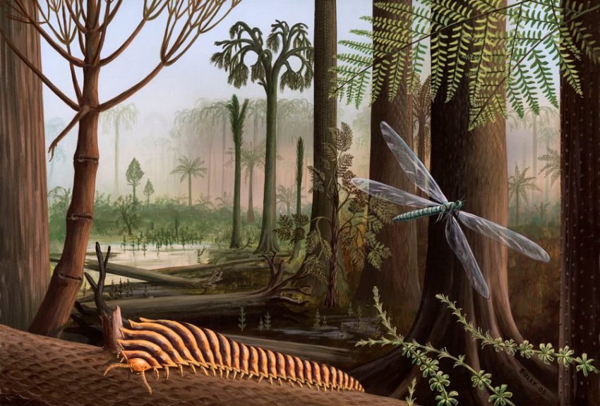
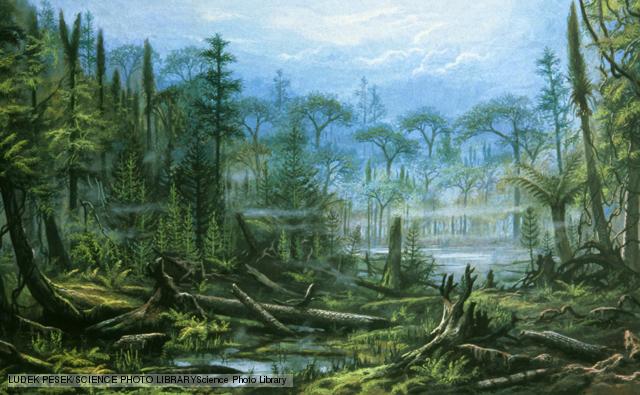
The presence of oxygen in the atmosphere had another major bene t for an organism trying to live at or above the surface: it ltered ultraviolet radiation. Ultraviolet radiation breaks down many molecules–from DNA and oxygen to the chlorouorocarbons that are implicated in stratospheric ozone depletion. Such energy splits oxygen into the highly unstable atomic form O, which can combine back into O2 and into the very special molecule O3, or ozone. Ozone, in turn, absorbs ultraviolet radiation. It was not until oxygen was abundant enough in the atmosphere to allow the formation of ozone that life even had a chance to get a root-hold or a foothold on land. It is not a coincidence that the rapid evolution of life from prokaryotes (single-celled organisms with no nucleus) to eukaryotes (single-celled organisms with a nucleus) to metazoa (multicelled organisms) took place in the billion-year-long era of oxygen and ozone.

Although the atmosphere was reaching a fairly stable level of oxygen during this period, the climate was hardly uniform. There were long stages of relative warmth or coolness during the transition to modern geologic time. The composition of fossil plankton shells that lived near the ocean oor provides a measure of bottom water temperatures. The record suggests that over the past 100 million years bottom waters cooled by nearly 15 degrees Celsius. Sea levels dropped by hundreds of meters, and continents drifted apart. Inland seas mostly disappeared, and the climate cooled an average of 10 to 15 degrees C. Roughly 20 million years ago permanent ice appears to have built up on Antarctica.

About two million to three million years ago the paleoclimatic record starts to show signi cant expansions and contractions of warm and cold periods in 40,000-year or so cycles. This periodicity is interesting because it corresponds to the time it takes Earth to complete an oscillation of the tilt of its axis of rotation. It has long been speculated, and recently calculated, that known changes in orbital geometry could alter the amount of sunlight coming in between winter and summer by about 10 percent or so and could be responsible for initiating or ending ice ages.

The warm hand of man

MOST INTERESTING and perplexing is the discovery that between 600,000 and 800,000 years ago the dominant cycle switched from 40,000-year periods to 100,000-year intervals with very large uctuations. The last major phase of glaciation ended about 10,000 years ago. At its height 20,000 years ago, ice sheets about two kilometers thick covered much of northern Europe and North America. Glaciers expanded in high plateaus and mountains throughout the world. Enough ice was locked up on land to cause sea levels to drop more than 100 meters below where they are today. Massive ice sheets scoured the land and revamped the ecological face of Earth, which was ve degrees C cooler on average than it is currently.

The precise causes of the longer intervals between warm and cold periods are not yet sorted out. Volcanic eruptions may have played a signi cant role, as shown by the effect of El Chichón in Mexico and Mount Pinatubo in the Philippines. Tectonic events, such as the development of the Himalayas, may have inuenced world climate. Even the impact of comets can inuence short-term climatic trends with catastrophic consequences for life [see “What Caused the Mass Extinction? An Extraterrestrial Impact,” by Walter Alvarez and Frank Asaro; and “What Caused the Mass Extinction? A Volcanic Eruption,” by Vincent E. Courtillot; Scientific American, October 1990]. It is remarkable that despite violent, episodic perturbations, the climate has been buffered enough to sustain life for 3.5 billion years.

One of the most pivotal climatic discoveries of the past 30 years has come from ice cores in Greenland and Antarctica. When snow falls on these frozen continents, the air between the snow grains is trapped as bubbles. The snow is gradually compressed into ice, along with its captured gases. Some of these records can go back more than 500,000 years; scientists can analyze the chemical content of ice and bubbles from sections of ice that lie as deep as 3,600 meters (2.2 miles) below the surface.

The ice-core borers have determined that the air breathed by ancient Egyptians and Anasazi Indians was very similar to that which we inhale today–except for a host of air pollutants introduced over the past 100 or 200 years. Principal among these added gases, or pollutants, are extra carbon dioxide and methane. Since about 1860–the expansion of the Industrial Revolution–carbon dioxide levels in the atmosphere have increased more than 30 percent as a result of industrialization and deforestation; methane levels have more than doubled because of agriculture, land use and energy production. The ability of increased amounts of these gases to trap heat is what drives concerns about climate change in the 21st century [see “The Changing Climate,” by Stephen H. Schneider; Scientific American, September 1989].

The ice cores have shown that sustained natural rates of worldwide temperature change are typically about one degree C per millennium. These shifts are still signi cant enough to have radically altered where species live and to have potentially contributed to the extinction of such charismatic megafauna as mammoths and saber-toothed tigers. But a most extraordinary story from the ice cores is not the relative stability of the climate during the past 10,000 years. It appears that during the height of the last ice age 20,000 years ago there was 50 percent less carbon dioxide and less than half as much methane in the air than there has been during our epoch, the Holocene. This nding suggests a positive feedback between carbon dioxide, methane and climatic change.

The reasoning that supports the idea of this destabilizing feedback system goes as follows. When the world was colder, there was less concentration of greenhouse gases, and so less heat was trapped. As Earth warmed up, carbon dioxide and methane levels increased, accelerating the warming. If life had a hand in this story, it would have been to drive, rather than to oppose, climatic change. It appears increasingly likely that when humans became part of this cycle, they, too, helped to accelerate warming. Such warming has been especially pronounced since the mid-1800s because of greenhouse gas emissions from industrialization, land-use change and other phenomena. Once again, though, uncertainties remain.

Nevertheless, most scientists would agree that life could well be the principal factor in the positive feedback between climatic change and greenhouse gases. There was a rapid rise in average global surface temperature at the end of the 20th century [see illustration on opposite page]. Indeed, the period from the 1980s onward has been the warmest of the past 2,000 years. Nineteen of the 20 warmest years on record have occurred since 1980, and the 12 warmest have all occurred since 1990. The all-time record high year was 1998, and 2002 and 2003 were in second and third places, respectively. There is good reason to believe that the decade of the 1990s would have been even hotter had not Mount Pinatubo erupted: this volcano put enough dust into the high atmosphere to block some incident sunlight, causing global cooling of a few tenths of a degree for several years.

Could the warming of the past 140 years have occurred naturally? With ever increasing certainty, the answer is no.

The box at the right shows a remarkable study that attempted to push back the Northern Hemisphere’s temperature record a full 1,000 years. Climatologist Michael Mann of the University of Virginia and his colleagues performed a complex statistical analysis involving some 112 different factors related to temperature, including tree rings, the extent of mountain glaciers, changes in coral reefs, sunspot activity and volcanism.

The resulting temperature record is a reconstruction of what might have been obtained had thermometer-based measurements been available. (Actual temperature measurements are used for the years after 1860.) As shown by the confidence range, there is considerable uncertainty in each year of this 1,000-year temperature reconstruction. But the overall trend is clear: a gradual temperature decrease over the first 900 years, followed by a sharp temperature upturn in the 20th century. This graph suggests that the decade of the 1990s was not only the warmest of the century but of the entire past millennium.

By studying the transition from the high carbon dioxide, low-oxygen atmosphere of the Archean to the era of great evolutionary progress about half a billion years ago, it becomes clear that life may have been a factor in the stabilization of climate. In another example–during the ice ages and interglacial cycles–life seems to have the opposite function: accelerating the change rather than diminishing it. This observation has led one of us (Schneider) to contend that climate and life coevolved rather than life serving solely as a negative feedback on climate.

If we humans consider ourselves part of life–that is, part of the natural system–then it could be argued that our collective impact on Earth means we may have a signi cant co-evolutionary role in the future of the planet. The current trends of population growth, the demands for increased standards of living and the use of technology and organizations to attain these growth-oriented goals all contribute to pollution. When the price of polluting is low and the atmosphere is used as a free sewer, carbon dioxide, methane, chlorouorocarbons, nitrous oxides, sulfur oxides and other toxics can build up.

Drastic changes ahead

IN THEIR REPORT Climate Change 2001, climate experts on the Intergovernmental Panel on Climate Change estimated that the world will warm between 1.4 and 5.8 degrees C by 2100. The mild end of that range–a warming rate of 1.4 degrees C per 100 years–is still 14 times faster than the one degree C per 1,000 years that historically has been the average rate of natural change on a global scale. Should the higher end of the range occur, then we could see rates of climatic change nearly 60 times faster than natural average conditions, which could lead to changes that many would consider dangerous. Change at this rate would almost certainly force many species to attempt to move their ranges, just as they did from the ice age/interglacial transition between 10,000 and 15,000 years ago. Not only would species have to respond to climatic change at rates 14 to 60 times faster, but few would have undisturbed, open migration routes as they did at the end of the ice age and the onset of the interglacial era. The negative effects of this significant warming–on health, agriculture, coastal geography and heritage sites, to name a few–could also be severe.

To make the critical projections of future climatic change needed to understand the fate of ecosystems on Earth, we must dig through land, sea and ice to learn as much from geologic, paleoclimatic and paleoecological records as we can. These records provide the backdrop against which to calibrate the crude instruments we must use to peer into a shadowy environmental future, a future increasingly inuenced by us.

THE AUTHORS

CLAUDE J. ALLGRE and STEPHEN H. SCHNEIDER study various aspects of Earths geologic history and its climate. Allgre is professor at the University of Paris and directs the department of geochemistry at the Paris Geophysical Institute. He is a foreign member of the National Academy of Sciences. Schneider is professor in the department of biological sciences at Stanford University and co-director of the Center for Environmental Science and Policy. He was honored with a MacArthur Prize Fellowship in 1992 and was elected to membership in the National Academy of Sciences in 2002.

This article was originally published with the title “Evolution of Earth” on www.scientificamerican.com (2005)

Fossils

Saturday, November 19, 2016

Fossils are evidence of ancient life forms or ancient habitats which have been preserved by natural processes. They can be the actual remains of a once living thing, such as bones or seeds, or even traces of past events such as dinosaur footprints, or the ripple marks on a prehistoric shore. Geologists can tell the age of a fossil through a variety of radiometric dating techniques. The breakdown of radioactive isotopes of certain elements, such as carbon, uranium and potassium takes place at a known rate, so the age of a rock or mineral containing these isotopes can be calculated.

History of paleontology

People have been fascinated by fossils for thousands of years, and as long ago as ancient Greek times were correctly interpreting them as the remains of long dead creatures. Palaeontology began to be formalised and treated with scientific rigour from the 17th century onwards. At this time, people started to calculate the age of the Earth and get to grips with the fact that the extinction of a whole species was not only possible, but had occurred many times already. The publication of Darwin’s ‘On the Origin of Species’ in the mid-19th century gave new impetus to palaeontology, as patterns and trends in evolution and extinction were eagerly sought and studied. Modern palaeontologists have an array of tools and processes at their fingertips, from sophisticated dating techniques to electron microscopes and medical scanners.

Diplodocus (left) lived during the Upper Jurassic period 159 to 144 million years ago. Triceratops lived during the Upper Cretaceous period 98-65 million years ago.

Fossil types

Body fossils are the preserved remains of the actual body parts of an animal or plant such as a skeleton or a pollen grain. Trace fossils are the remains of ancient activity, such as the burrow left by a worm or a stone tool made by a prehistoric person. Some fossils preserve original features in exquisite detail, while others are much cruder remnants.

How fossils are formed

Fossilization only happens in the rarest of cases, when a plant or animal dies in the right circumstances. Animal corpses are usually eaten by something, or bacteria rots them away before fossilization can occur, and even hard parts like bones and shells are eventually destroyed through erosion and corrosion. The trick to becoming a fossil is to die in a location where your body – or bits of it – are protected from scavengers and the elements. This means getting buried in sand, soil or mud and the best place for that is on the seabed or a river bed.

Only in very rare cases do the soft parts of animals – the flesh, skin and internal organs – become fossils. Even when buried under mud or soil, decay still takes place, though lack of oxygen does slow it down. If a skeleton is dug up at this stage, it will still be made of bone. Remains like these that haven’t truly fossilized yet are sometimes called ‘sub-fossils’.

As more time passes, sub-fossils become buried deeper and deeper. What was mud or sand becomes compressed on its way to becoming rock. But even safely sealed away underground, time doesn’t stand still. Chemicals and minerals percolate through the sediment and the original bone or shell gradually recrystallizes. In extreme cases, the entire thing can dissolve away, leaving a hollow where it once was. If paleontologists find a hollow like this, they can pour liquid rubber in to make a fossil cast, or put it in a medical scanner to see what the original looked like.

In other cases, minerals from the rocks gradually impregnate the bone, shell or wood, changing its chemical composition and making it capable of surviving for as long as – or sometimes longer than – the rock enclosing it. In cases where the original has dissolved away, the minerals can gradually fill the hollow to create a natural cast of the original. So sometimes a fossil doesn’t contain anything of the original creature except its shape. Even that shape can take a battering! If the rocks are distorted and squeezed by geological forces, then the fossils within them will be too.

Even rocks have a finite lifespan. Eventually the rock enclosing a fossil is eroded away, and the fossil is revealed on the surface of the ground. With luck, a sharp-eyed fossil collector will spot and excavate it. Otherwise the elements will continue to batter it, until it – along with the rocks around it – is reduced once more to sand, silt or mud.

Source: BBC/Nature

Impact Events

Saturday, November 19, 2016

Impact events, proposed as causes of mass extinction, are when the planet is struck by a comet or meteor large enough to create a huge shock wave felt around the globe. Widespread dust and debris rain down, disrupting the climate and causing extinction on a global, rather than local, scale. The demise of the dinosaurs at the end of the Cretaceous has been linked to an impact that left a crater in the seabed off the Yucatan peninsula of Mexico. Impacts have also been blamed for other mass extinctions, but the timing and links between cause and effect for these is still debated by scientists.

Chicxulub crater

The Chicxulub crater is an impact crater buried underneath the Yucatán Peninsula in Mexico. Its center is located near the town of Chicxulub, after which the crater is named. It was formed by a large asteroid or comet at least 10 kilometres (6 miles) in diameter, the Chicxulub impactor, striking the Earth. The date of the impact coincides precisely with the Cretaceous–Paleogene boundary (K–Pg boundary), around 66 million years ago, and a widely accepted theory is that worldwide climate disruption from the event was the cause of the Cretaceous–Paleogene extinction event, a mass extinction in which 75% of plant and animal species on Earth suddenly became extinct, including the dinosaurs. The crater is more than 180 kilometers (110 miles) in diameter and 20 km (12 mi) in depth, well into the continental crust of the region of about 10–30 km depth. It makes the feature the third of the largest confirmed impact structures on Earth.

Location of Chicxulub crater, Mexico

The crater was discovered by Antonio Camargo and Glen Penfield, geophysicists who had been looking for petroleum in the Yucatán during the late 1970s. Penfield was initially unable to obtain evidence that the geological feature was a crater and gave up his search. Later, through contact with Alan Hildebrand in 1990, Penfield obtained samples that suggested it was an impact feature. Evidence for the impact origin of the crater includes shocked quartz, a gravity anomaly, and tektites in surrounding areas.

In 2016, a scientific drilling project drilled deep into the peak ring of the impact crater, hundreds of meters below the current sea floor, to obtain rock core samples from the impact itself. The discoveries were widely seen as confirming current theories related to both the crater impact and its effects.

Imaging from NASA's Shuttle Radar Topography Mission STS-99 reveals part of the 180 km (110 mi) diameter ring of the crater. The numerous cenotes (sinkholes) clustered around the trough of the crater suggest a prehistoric oceanic basin in the depression left by the impact.

In 1978, geophysicists Glen Penfield and Antonio Camargo were working for the Mexican state-owned oil company Petróleos Mexicanos, or Pemex, as part of an airborne magnetic survey of the Gulf of Mexico north of the Yucatán Peninsula. Penfield's job was to use geophysical data to scout possible locations for oil drilling. In the offshore magnetic data, Penfield noted anomalies whose depth he estimated, and mapped. He then obtained onshore gravity data from the 1940s. According to Penfield, "The old data showed a large concentric set of onshore gravity anomalies. When I laid it next to my No. 2 pencil mapping of the offshore magnetic anomalies, the fit was perfect: a shallow, 180-kilometer diameter gravity-magnetic bullseye on the almost non-magnetic, uniform carbonate background of the Yucatan platform! We recognized the crater as the likely Cretaceous-Paleogene boundary event." A decade earlier, the same map suggested an impact feature to contractor Robert Baltosser, but he was forbidden to publicize his conclusion by Pemex corporate policy of the time.

Researchers at the University of Glasgow dated tektite samples from the impact as 66,038,000 ± 11,000 years old.

The Chicxulub impactor had an estimated diameter of 11–81 kilometers (6.8–50.3 mi), and delivered an estimated energy of 21–921 billion Hiroshima A-bombs. For comparison, this is ~100 million times the energy released by the Tsar Bomba, a thermonuclear device ("H-bomb") that remains the most powerful man-made explosive ever detonated, which released 210 petajoules or 50 megatons TNT). The impact created a hole 100 kilometers (62 mi) wide and 30 kilometers (19 mi) deep, leaving a crater mainly under the sea and covered by 600 meters (2,000 ft) of sediment by the 21st century.

Gravity anomaly map of the Chicxulub impact area. The coastline is shown as a white line. A series of concentric features reveals the location of the crater. White dots represent cenotes (water-filled sinkholes). A ring of cenotes is associated with the largest semicircular feature, although its exact origin remains unclear.

In their 1991 paper, Hildebrand, Penfield and company described the geology and composition of the impact feature. The rocks above the impact feature are layers of marl and limestone reaching to a depth of almost 1,000 m (3,300 ft). These rocks date back as far as the Paleocene. Below these layers lie more than 500 m (1,600 ft) of andesite glass and breccia. These andesitic igneous rocks were only found within the supposed impact feature, as is shocked quartz. The K–Pg boundary inside the feature is depressed to 600 to 1,100 m (2,000 to 3,600 ft) compared with the normal depth of about 500 m (1,600 ft) measured 5 km (3 mi) away from the impact feature.

Along the edge of the crater are clusters of cenotes or sinkholes, which suggest that there was a water basin inside the feature during the Neogene period, after the impact. The groundwater of such a basin would have dissolved the limestone and created the caves and cenotes beneath the surface. The paper also noted that the crater seemed to be a good candidate source for the tektites reported at Haiti.

Astronomical origin of asteroid

In September 2007, a report published in Nature proposed an origin for the asteroid that created the Chicxulub crater. The authors, William F. Bottke, David Vokrouhlický, and David Nesvorný, argued that a collision in the asteroid belt 160 million years ago resulted in the Baptistina family of asteroids, the largest surviving member of which is 298 Baptistina. They proposed that the "Chicxulub asteroid" was also a member of this group. The connection between Chicxulub and Baptistina is supported by the large amount of carbonaceous material present in microscopic fragments of the impactor, suggesting the impactor was a member of a rare class of asteroids called carbonaceous chondrites, like Baptistina. According to Bottke, the Chicxulub impactor was a fragment of a much larger parent body about 170 km (106 mi) across, with the other impacting body being around 60 km (37 mi) in diameter.

In 2011, new data from the Wide-field Infrared Survey Explorer revised the date of the collision which created the Baptistina family to about 80 million years ago. This makes an asteroid from this family highly improbable to be the asteroid that created the Chicxulub crater, as typically the process of resonance and collision of an asteroid takes many tens of millions of years. In 2010, another hypothesis was offered which implicated the newly discovered asteroid P/2010 A2, a member of the Flora family of asteroids, as a possible remnant cohort of the K/Pg impactor.

The center of the crater is near the village of Chicxulub Puerto, Yucatán.

Multiple impact hypothesis

In recent years, several other craters of around the same age as Chicxulub have been discovered, all between latitudes 20°N and 70°N. Examples include the disputed Silverpit crater in the North Sea, and the Boltysh crater in Ukraine. Both are much smaller than Chicxulub, but are likely to have been caused by objects many tens of meters across striking the Earth. This has led to the hypothesis that the Chicxulub impact may have been only one of several impacts that happened nearly at the same time. Another possible crater thought to have been formed at the same time is the larger Shiva crater, though the structure's status as an impact crater is contested.

The collision of Comet Shoemaker–Levy 9 with Jupiter in 1994 demonstrated that gravitational interactions can fragment a comet, giving rise to many impacts over a period of a few days if the comet should collide with a planet. Comets undergo gravitational interactions with the gas giants, and similar disruptions and collisions are very likely to have occurred in the past. This scenario may have occurred on Earth at the end of the Cretaceous, though Shiva and the Chicxulub craters might have been formed 300,000 years apart.

In late 2006, Ken MacLeod, a geology professor from the University of Missouri, completed an analysis of sediment below the ocean's surface, bolstering the single-impact theory. MacLeod conducted his analysis approximately 4,500 kilometers (2,800 mi) from the Chicxulub crater to control for possible changes in soil composition at the impact site, while still close enough to be affected by the impact. The analysis revealed there was only one layer of impact debris in the sediment, which indicated there was only one impact. Multiple-impact proponents such as Gerta Keller regard the results as "rather hyper-inflated" and do not agree with the conclusion of MacLeod's analysis, arguing that there might only be gaps of hours to days between impacts in a multiple-impact scenario (cf. Shoemaker-Levy 9) which would not leave a detectable gap in deposits.

Source: https://en.wikipedia.org

Pages